Quantum Computing for Computer Engineers - Part 1

Qubits and quantum gates

Here’s the thing about Quantum Computing: it is one of the most interesting and promising fields of research, but at the same time one of the most obscure. The idea of building a computer using the sometimes counter-intuitive laws of quantum mechanics is quite old, and since the 80s people are developing a quantum computation theory. One of the first reasons why this could be relevant is the inherent difficulty of simulating quantum systems on classical computers (as pointed out by Feynman himself in 1982). Secondly, a computer built using the rules of quantum mechanics can, in theory, solve a particular set of problems way faster than a standard computer. For example, it could search an element in a generic vector in \(O(\sqrt{n})\)!

Quantum computers are not only theoretical devices, they actually exist and have been built by companies in the quest of developing this new and completely different technology. Demonstrating that a quantum computer can solve a problem more efficiently than a standard computer, however, is not an easy task, this is the so called quantum supremacy problem. In a paper from 2019, Google announced that it had achieved for the first time quantum supremacy. Since then, papers were published showing how the results claimed by Google were beaten using new techniques to simulate quantum computers on standard supercomputers. Competition is fierce and the quest to find quantum algorithms able to outperform standard computers is still on.

This article is the first of a series of posts in which we are going to introduce the basis of quantum computing theory, with some examples and a little bit of math. The article is meant for people with a general knowledge of linear algebra and computer science, but zero knowledge of quantum physics. Oftentimes, introductory explanations on quantum computing are either too basic, using simplifying metaphors that don’t really correspond to how things actually work, or too advanced, cluttering the reader with a mathematical overhead that is not really required to understand and use these concepts, at least at first. Our purpose is to bridge the divide between these two explanations, giving you a clear picture of these abstract concepts while reducing the math to an accessible amount.

The Qubit

Let’s start with the basics. In classical theory of computation, the basic element is the bit, it’s a simple object that can assume either value \(0\) or \(1\). Well, in quantum we have an analogous: the quantum bit or qubit for short. Just as the standard bit has two states: \(0\) and \(1\) a qubit can have two states: \(\ket{0}\) and \(\ket{1}\). We represent these simple states with 2-element vectors. The weird \(\ket{\cdot}\) notation is a short way of representing a vector and is called the Dirac notation. Our base states are thus:

\[\ket{0} = \begin{bmatrix} 1 \\ 0 \end{bmatrix}\;\; \ket{1} = \begin{bmatrix} 0 \\ 1 \end{bmatrix}\]

The thingy about qubits is that they can be in states other than \(\ket{0}\) or \(\ket{1}\). In fact, they can be in any linear combinations of these states, also known as superpositions:

\[\ket{\psi} = \alpha\ket{0} + \beta\ket{1} = \alpha\begin{bmatrix} 1 \\ 0 \end{bmatrix} + \beta\begin{bmatrix} 0 \\ 1 \end{bmatrix} = \begin{bmatrix} \alpha \\ \beta \end{bmatrix}\]

where \(\alpha\) and \(\beta\) are two complex numbers. For now you can think of them as real numbers, you’ll see that not much is lost. In math terms, you can see a qubit as a vector in a 2-D space, where the special states \(\ket{0}\) and \(\ket{1}\) are the so called computational basis states.

Pretty easy until now, right? Well it turns out that qubit have another relevant difference with their classical counterpart. When reading the value of a bit this can be in just two states: either \(0\) or \(1\). When we try to read a qubit (also called measurement) we find that we can not retrieve directly its values \(\alpha\) and \(\beta\), also in this case we only get either a \(0\) or \(1\). So where is the difference? While classical bits always exist in some definite state, qubits in superposition exist in multiple states at the same time. This is counter-intuitive and pretty far from what we observe in our daily lives. This does not mean that qubits are secretly in some state we don’t know until we take a look. This is an inherent property of nature: some things are not defined until they are measured. If we were to repeat a measurement multiple times we would observe that sometimes we land on \(0\) and sometimes we land on \(1\), with probabilities \(|\alpha|^2\) and \(|\beta|^2\) respectively. A qubit can be seen as a “list” of probabilities of its outcomes (more properly called distribution). Since probabilities sum to \(1\), we find that for all qubits:

\[|\alpha|^2+|\beta|^2=1\]

For example let’s consider the following qubits:

\[\ket{A} = \begin{bmatrix} \frac{1}{\sqrt{2}} \\[5pt] -\frac{1}{\sqrt{2}} \end{bmatrix} \longrightarrow \Big| \frac{1}{\sqrt{2}} \Big|^2 + \Big|-\frac{1}{\sqrt{2}}\Big|^2 = 1\] \[\ket{B} = \begin{bmatrix} 1 \\[5pt] 1 \end{bmatrix} \longrightarrow 2 \neq 1\]

Notice how in the example shown above, \(\ket{A}\) is a valid qubit, while \(\ket{B}\) is not, since its values don’t sum to \(1\). Also observe how values inside state vectors can be negative and still produce valid probabilities (we are taking a squared norm, after all).

Observe also how qubits can encode values that have an infinite number of decimal digits at no extra cost. If we keep qubits in superposition we have an infinite precision representation of numbers:

\[\ket{A} = \begin{bmatrix} \frac{1}{\sqrt{2}} \\[5pt] -\frac{1}{\sqrt{2}} \end{bmatrix} = \begin{bmatrix} 0.7071... \\[5pt] -0.7071... \end{bmatrix}\]

How great this is! But as soon as we measure a qubit, some part of it is lost. We go from a potentially infinite amount of information to a single bit. This means there is a sort of hidden information encoded somewhere, but we can see just a part of it. This information actually exists and we can perform computations with it (this is the whole point of quantum computing). In a nutshell, the goal of quantum computing is to find clever ways to extract this hidden information in the most efficient way possible.

A useful analogy for understanding the qubit is the Schrödinger’s cat (if you don’t know about this thought experiment, more info can be found here). To recap what the experiment is about: let’s imagine to put a cat, a flask of poison and a source of radiation in a box. The source of radiation is an atom in a superposition of \(\ket{decayed}\) and \(\ket{not\,decayed}\). If a Geiger counter detects radioactivity it causes the release of poison, thus killing the cat. The point is that we don’t know when the Geiger counter will detect radioactivity (n.d.r. caused by a single atom decaying). So if we close the box we don’t know if the cat it’s still alive or dead. We can say that the cat is in a superposition of these states, being both alive and dead at the same time, like a qubit can be both \(\ket{0}\) and \(\ket{1}\). The point is that, when we eventually open the box, the cat can not be in a mixture of the two states, it will be alive or dead, exactly how the qubit, when measured, can just be \(0\) or \(1\). Why does this state collapse happens? Nobody knows, but this is how things work, you know.

Back to our math, we said that the values \(|\alpha|^2+|\beta|^2=1\), so a qubit can be seen as a unit vector in a two dimensional complex space, thus we may rewrite the qubit as:

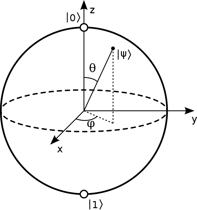
\[\ket{\psi}=e^{i\gamma}\left(\cos\frac{\theta}{2}\ket{0}+e^{i\varphi}\sin\frac{\theta}{2}\ket{1}\right)\]

with \(\theta\), \(\varphi\), \(\gamma\) real numbers. Actually we can ignore the factor \(e^{i\gamma}\) (the reason why is outside the scope of this article), thus rewriting the qubit as:

\[\ket{\psi}=\cos\frac{\theta}{2}\ket{0}+e^{i\varphi}\sin\frac{\theta}{2}\ket{1}\]

We can see the qubit as a point in the 3-D unit sphere, also called Bloch sphere, this visualization is often used in quantum computing, even if it can not be generalized to multiple qubit systems.

Figure 1: A Bloch sphere

Quantum Gates

We have our qubit, the basic quantum computational element, now we should introduce how to use it. Simple! We can use quantum gates: just as classical computers have logical gates to manipulate information, quantum computers have quantum gates. Let’s keep it simple for now and consider just single bit gates. In classical computation theory the only interesting single bit gate is the NOT, providing the mapping \(0\to1\), \(1\to0\). There are also three other single bit gates: Identity, Set to \(0\) and Set to \(1\), but they are not that interesting.

Can we imagine an analogous quantum NOT gate? This would be a gate that inverts the state \(\ket{0}\) to \(\ket{1}\) and vice versa. The problem here is that specifying an action on the states \(\ket{0}\) and \(\ket{1}\) does not tell anything about what happens to the superposition of these two states. The quantum NOT on the other hand acts linearly, this means that it takes a qubit in the state:

\[\ket{\psi} = \alpha\ket{0} + \beta\ket{1}\]

and outputs the qubit:

\[\ket{\psi} = \beta\ket{0} + \alpha\ket{1}\]

Actually all quantum gates, not just the NOT, act in a linear fashion. This is a general property of quantum operators. Since a quantum gate acts linearly, we can represent it in a matrix form. For example, here is the quantum NOT we described earlier:

\[X = \begin{bmatrix} 0 & 1\\ 1 & 0 \end{bmatrix}\]

This is how the gate operates in matricial form:

\[X\begin{bmatrix}\alpha \\ \beta\end{bmatrix} = \begin{bmatrix} 0 & 1\\ 1 & 0 \end{bmatrix} \begin{bmatrix}\alpha \\ \beta\end{bmatrix} = \begin{bmatrix}\beta \\ \alpha\end{bmatrix}\]

That’s quite interesting: we can describe quantum gates by matrices, but what are the property that these matrices should have? Well, for every qubit with parameters \(\alpha\) and \(\beta\) we have the constraint \(|\alpha|^2+|\beta|^2=1\), this means that if we let our valid qubit go through a quantum gate then we want a valid qubit on the way out, with squared values that sum to 1. With a little bit of linear algebra it is possible to show that for a matrix \(U\) to be a valid quantum gate it should have the property: \(U^{\dagger}U=I\). \(U^{\dagger}\) is the adjoint matrix of \(U\) (also called Hermitian transpose), obtained by taking the transpose of \(U\) and complex conjugating it. This constraint is called Hermiticity, and any matrix that satisfies it is a valid quantum gate! This means that there many non-trivial single bit quantum gates.

For example a very important gate is the Hadamard gate:

\[H = \frac{1}{\sqrt{2}}\begin{bmatrix} 1 & 1 \\ 1 & -1 \end{bmatrix}\]

This gate sends states in superposition. Observe below how, by feeding it a base state \(\ket{0}\) or \(\ket{1}\), we are left with a superposition with a \(50\%\) chance of landing on \(0\) and a \(50\%\) chance of landing on \(1\).

\[H\begin{bmatrix}1 \\ 0\end{bmatrix} = \begin{bmatrix}\frac{1}{\sqrt{2}} \\[5pt] \frac{1}{\sqrt{2}}\end{bmatrix}\] \[H\begin{bmatrix}0 \\ 1\end{bmatrix} = \begin{bmatrix}\frac{1}{\sqrt{2}} \\[5pt] -\frac{1}{\sqrt{2}}\end{bmatrix}\] \[\Big| \frac{1}{\sqrt{2}} \Big|^2 = \Big|-\frac{1}{\sqrt{2}}\Big|^2 = 0.5\]

A natural question to ask is: why the \(-1\) in the bottom right corner of the matrix? This is because an important property of quantum gates (derived from the Hermiticity constraint) is that all gates should be reversible, i.e. if we let the output qubit go through the same gate we will end up with the original one. This is actually an important property of quantum phisics that emerges in multiple situations.

Conclusion

In this introductory article we gave you a taste of quantum computing and we introduced some fundamental concepts and notation. Probably you’ll be quite confused at this point. Don’t worry, it’s normal. Quantum computing is hard to grasp at first, but if you decide to delve deeper into it, things will make more and more sense. There are many reasons for doing so: one can be personal interest, another can be the fact that investing time in learning these concepts can be very strategic. Many large companies have invested millions into this field, and breakthroughs happen by the day. Whatever your reason, if you want to go deeper we published on our blog a part 2 of this article. Here we kept the math simple and intuitive, while in part 2 we focus more on the math formalism and introduce some other important concepts. Don’t be scared: if you have a general knowledge of computer science and linear algebra you’ll be able to follow it!

Sources

Nielsen, M., & Chuang, I. (2010). Quantum Computation and Quantum Information: 10th Anniversary Edition. Cambridge: Cambridge University Press. doi:10.1017/CBO9780511976667